Sensor Offset Prediction

Libraries

from sklearn.model_selection import KFold, cross_validate, cross_val_score, cross_val_predict  # train_test_split,
from sklearn.preprocessing import StandardScaler
from sklearn.utils import resample

from sklearn.ensemble import RandomForestClassifier
from sklearn.tree import DecisionTreeClassifier
from sklearn.neighbors import KNeighborsClassifier
from sklearn.linear_model import LogisticRegression
from sklearn.impute import KNNImputer

from sklearn.model_selection import GridSearchCV

from sklearn.pipeline import Pipeline
from sklearn.compose import ColumnTransformer


from sklearn.metrics import accuracy_score, confusion_matrix, classification_report, ConfusionMatrixDisplay, precision_score, recall_score

Feature Engineering

For the training set all missing values will be removed from the data.
Additional variables such as an ordinal air quality index (as integer) for both sensors will be added to the training set.
Also the hour and day of the year will be extracted from the datetime variable after which the datetime variable will be dropped with the Id variable as they are both features with high cardinality.

ord_train = train.sort_values(by="Datetime")

add_df = cfun.add_attributes(ord_train, drop_nan_value=True, fill_nan_value=False)

train_c = add_df.drop_missing_value()
train_c = add_df.add_air_quality_index()
train_c = add_df.add_period_variables(hour=True, dayofyear=True)
train_c = train_c.drop(["ID", "Datetime"], axis = 1)

train_c.info()

C:\Users\AYOMIDE\vs-python\PM_ML_project\function.py:237: FutureWarning: Series.dt.weekofyear and Series.dt.week have been deprecated. Please use Series.dt.isocalendar().week instead.

<class 'pandas.core.frame.DataFrame'>
Int64Index: 290014 entries, 116880 to 226302
Data columns (total 9 columns):
 #   Column             Non-Null Count   Dtype  
---  ------             --------------   -----  
 0   Sensor1_PM2.5      290014 non-null  float64
 1   Sensor2_PM2.5      290014 non-null  float64
 2   Temperature        290014 non-null  float64
 3   Relative_Humidity  290014 non-null  float64
 4   Offset_fault       290014 non-null  int64  
 5   S1_AQI             290014 non-null  int64  
 6   S2_AQI             290014 non-null  int64  
 7   Hour               290014 non-null  int64  
 8   Day_Of_Year        290014 non-null  int64  
dtypes: float64(4), int64(5)
memory usage: 22.1 MB

Separating the label for the predictors.

outcome = "Offset_fault"
X = train_c.drop(outcome, axis = 1)
y = train_c[outcome]

feature_names = list(train_c.drop(outcome, axis = 1).columns)

Scale all numeric features

num_features = list(X.select_dtypes("number").columns)
num_pipeline = Pipeline([
    ("std_scaler", StandardScaler())
])

full_pipeline = ColumnTransformer([
    ("num", num_pipeline, num_features)
])

X = full_pipeline.fit_transform(X)

X

array([[-1.10957703, -1.01101351,  1.71196075, ...,  1.66087637,
         0.66730492,  0.20484599],
       [-1.08300205, -0.94242651,  1.71196075, ...,  1.66087637,
         0.66730492,  0.20484599],
       [-1.20189013, -1.22443398,  1.71196075, ...,  1.66087637,
         0.66730492,  0.20484599],
       ...,
       [ 0.11881666,  0.48919661, -1.67174045, ..., -0.52823302,
        -0.62421669, -1.84915195],
       [ 0.27721755,  0.2761243 , -1.67174045, ..., -0.52823302,
        -0.62421669, -1.84915195],
       [-0.01650596, -0.22243706, -1.67174045, ...,  0.56632168,
        -0.62421669, -1.84915195]])

Inital Selected Models

Multiple models will be used to _see the best that generalize well on the validation set.

log_reg = LogisticRegression(random_state=11)
dt_class = DecisionTreeClassifier(random_state=11)
rf_class = RandomForestClassifier(random_state=11, n_jobs=-1)
knn_class = KNeighborsClassifier(n_jobs=-1)

model = [log_reg, dt_class, rf_class, knn_class]
model_names = ["Logistic Regression", "Decision Tree", "Random Forest", "K-Neighbors"]

Cross Validation

def cross_validation(model, x=X, y=y, model_name="model", cv=5):
    y_pred = cross_val_predict(model, x, y, cv=cv, n_jobs=-1) 
        
    print(f"{model_name}\n{'='*50}")
    
    print(f"Confusion Matrix ::-\n{confusion_matrix(y, y_pred)}")
    print(50*"-","\n")
    print(f"Accuracy :: {accuracy_score(y, y_pred)}\n")
    print(classification_report(y, y_pred))

For better model performance evaluation the training set will be divided into a smaller training set and a validation set (default will be 5 splits).

for mdl, mdl_name in zip(model, model_names):
    cross_validation(mdl, model_name=mdl_name)
    print("\n\n")

Logistic Regression
==================================================

Confusion Matrix ::-
[[171446  11417]
 [ 25463  81688]]
-------------------------------------------------- 

Accuracy :: 0.8728337252684353

              precision    recall  f1-score   support

           0       0.87      0.94      0.90    182863
           1       0.88      0.76      0.82    107151

    accuracy                           0.87    290014
   macro avg       0.87      0.85      0.86    290014
weighted avg       0.87      0.87      0.87    290014

Decision Tree
==================================================
Confusion Matrix ::-
[[162400  20463]
 [ 19569  87582]]
-------------------------------------------------- 

Accuracy :: 0.8619652844345446

              precision    recall  f1-score   support

           0       0.89      0.89      0.89    182863
           1       0.81      0.82      0.81    107151

    accuracy                           0.86    290014
   macro avg       0.85      0.85      0.85    290014
weighted avg       0.86      0.86      0.86    290014

Random Forest
==================================================
Confusion Matrix ::-
[[165178  17685]
 [ 15173  91978]]
-------------------------------------------------- 

Accuracy :: 0.8867020212817313

              precision    recall  f1-score   support

           0       0.92      0.90      0.91    182863
           1       0.84      0.86      0.85    107151

    accuracy                           0.89    290014
   macro avg       0.88      0.88      0.88    290014
weighted avg       0.89      0.89      0.89    290014

K-Neighbors
==================================================
Confusion Matrix ::-
[[158818  24045]
 [ 39627  67524]]
-------------------------------------------------- 

Accuracy :: 0.7804519781803637

              precision    recall  f1-score   support

           0       0.80      0.87      0.83    182863
           1       0.74      0.63      0.68    107151

    accuracy                           0.78    290014
   macro avg       0.77      0.75      0.76    290014
weighted avg       0.78      0.78      0.78    290014

Out of all the inital selected models, The Random Forest model have the best performance when we look at it accuracy score in predicting sensor device signal offsets. The model also looks promising in generalizing well on other data.

def eval_gs(gs, output="best_estimator"):
    if output == "best_estimator":
        return gs.best_estimator_
    elif output == "best_param":
        return gs.best_params_
    elif output == "scores_table":
        cv_res = gs.cv_results_
        
        f_df = pd.DataFrame(cv_res["params"])
        f_df["mean_test_score"] = cv_res["mean_test_score"]
        f_df["rank_test_score"] = cv_res["rank_test_score"]
        f_df["mean_train_score"] = cv_res["mean_train_score"]
        return f_df.sort_values(by="rank_test_score", ascending=True)
    
    elif output == "feature_importance":
        feature_importances = grid_search.best_estimator_.feature_importances_
        feat_imp = pd.DataFrame(sorted(zip(feature_names, feature_importances), reverse=True), columns = ["importance_score", "Feature"])
        return feat_imp.sort_values(by = "Feature", ascending=False)
    else:
        raise ValueError("`output` variable was given a wrong value.")

Hyperparameter Tuning

Using multiple random forest parameters to train the model on the data, in oreder to get the best combination of hyperparameter values.

param_grid = {"n_estimators": [100, 200, 300], "max_leaf_nodes": [10, 16], 'max_features':[3, 4]}

grid_search = GridSearchCV(rf_class, param_grid, cv=4, n_jobs=-1, return_train_score=True)

grid_search.fit(X, y)

GridSearchCV(cv=4, estimator=RandomForestClassifier(n_jobs=-1, random_state=11),
             n_jobs=-1,
             param_grid={'max_features': [3, 4], 'max_leaf_nodes': [10, 16],
                         'n_estimators': [100, 200, 300]},
             return_train_score=True)

In a Jupyter environment, please rerun this cell to show the HTML representation or trust the notebook.
On GitHub, the HTML representation is unable to render, please try loading this page with nbviewer.org.

Best Estimators

eval_gs(grid_search)

RandomForestClassifier(max_features=4, max_leaf_nodes=16, n_jobs=-1,
                       random_state=11)

In a Jupyter environment, please rerun this cell to show the HTML representation or trust the notebook.
On GitHub, the HTML representation is unable to render, please try loading this page with nbviewer.org.

eval_gs(grid_search, "best_param")

{'max_features': 4, 'max_leaf_nodes': 16, 'n_estimators': 100}

eval_gs(grid_search, "scores_table")

	max_features	max_leaf_nodes	n_estimators	mean_test_score	rank_test_score	mean_train_score
9	4	16	100	0.835939	1	0.846201
10	4	16	200	0.834090	2	0.845402
11	4	16	300	0.831949	3	0.843678
3	3	16	100	0.809878	4	0.818747
4	3	16	200	0.807188	5	0.817267
5	3	16	300	0.807185	6	0.816305
6	4	10	100	0.805216	7	0.812193
7	4	10	200	0.797896	8	0.805109
8	4	10	300	0.797492	9	0.805243
0	3	10	100	0.781183	10	0.787738
2	3	10	300	0.777797	11	0.783745
1	3	10	200	0.777648	12	0.784164

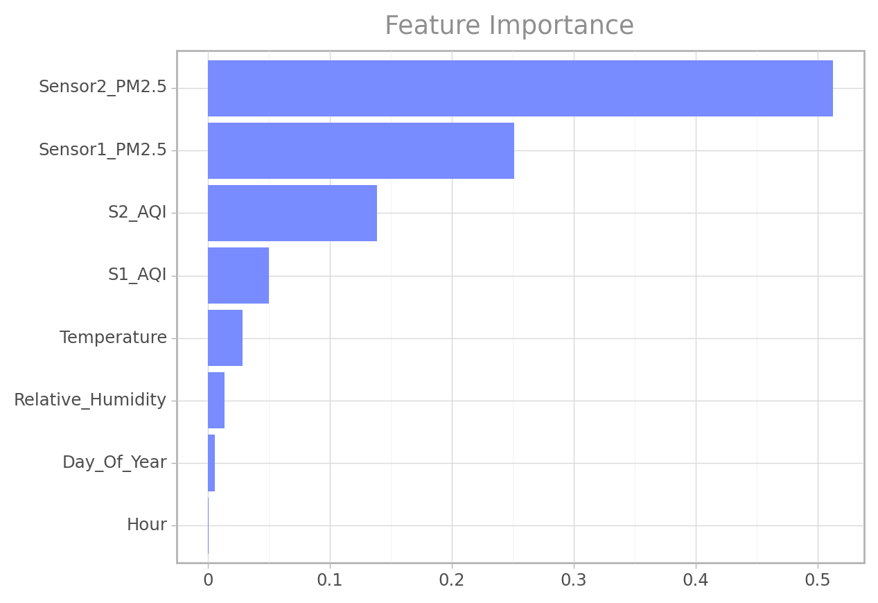
Feature Importance

Finding the relative importance of each feature for making accurate predictions.

ft_imp = eval_gs(grid_search, "feature_importance")
ft_imp

	importance_score	Feature
1	Sensor2_PM2.5	0.512644
2	Sensor1_PM2.5	0.250991
3	S2_AQI	0.138374
4	S1_AQI	0.049779
0	Temperature	0.028415
5	Relative_Humidity	0.013785
7	Day_Of_Year	0.005353
6	Hour	0.000660

(
    ggplot(ft_imp, aes(x="reorder(importance_score, Feature)", y="Feature")) +
    geom_col(fill="#788BFF") +
    coord_flip() +
    labs(x="", y="", title="Feature Importance") +
    theme_light() +
    theme(plot_title= element_text(color="#8F8F8F"))
)

<ggplot: (101708896235)>

Engineering The Test Set

All missing values will be imputed with their respective median value and all other feature transformation done on the train set will be used on the test set.

test = pd.read_csv('data/test.csv', parse_dates = ['Datetime'])

ord_test = test.sort_values(by="Datetime").reset_index(drop=True)

add_df = cfun.add_attributes(ord_test, drop_nan_value=False, fill_nan_value=True)

test_c = add_df.fill_missing_value(fill_fun = "median")
test_c = add_df.add_air_quality_index()
test_c = add_df.add_period_variables(hour=True, dayofyear=True)
test_c = test_c.drop(["ID", "Datetime"], axis = 1)

test_c = full_pipeline.transform(test_c)

C:\Users\AYOMIDE\vs-python\PM_ML_project\function.py:237: FutureWarning: Series.dt.weekofyear and Series.dt.week have been deprecated. Please use Series.dt.isocalendar().week instead.

final_model = grid_search.best_estimator_

final_prediction = final_model.predict(test_c)

samplesubmission = pd.read_csv('data/SampleSubmission.csv')

accuracy_score(samplesubmission["Offset_fault"], final_prediction)

0.7908621948634197

confusion_matrix(samplesubmission["Offset_fault"], final_prediction)

array([[100725,  26636],
       [     0,      0]], dtype=int64)

print(classification_report(samplesubmission["Offset_fault"], final_prediction))

              precision    recall  f1-score   support

           0       1.00      0.79      0.88    127361
           1       0.00      0.00      0.00         0

    accuracy                           0.79    127361
   macro avg       0.50      0.40      0.44    127361
weighted avg       1.00      0.79      0.88    127361

The test set seems to have an unusual task of predicting just one class which was the time the PM sensors where considered to have no offset faults. That been said, the model only detect that there were no fault in the sensor signals 79% of the time. Given that there are only 0s i.e non offset sensor signals we have a percision of 100%.

Saving Fitted Model

import pickle 

with open("pm2.5_sensor_offset.pkl", "wb") as f:
    pickle.dump(final_model, f)

Function to easily make future predictions

def make_predictions(data_file_path, model_file_path):
    """
    param: data_file_path : The file path to the new set of records.
    param: model_file_path: The file path to the pickle serialized file.

    return: pandas serise with predicted values.
    """

    # data transformation
    from function import add_attributes
    from pandas import Series
    ord_rec = test.sort_values(by="Datetime").reset_index(drop=True)

    add_df = add_attributes(ord_rec, drop_nan_value=False, fill_nan_value=True)

    rec_c = add_df.fill_missing_value(fill_fun = "median")
    rec_c = add_df.add_air_quality_index()
    rec_c = add_df.add_period_variables(hour=True, dayofyear=True)
    rec_c = rec_c.drop(["ID", "Datetime"], axis = 1)

    rec_c = full_pipeline.transform(rec_c)

    # Load model
    with open(model_file_path, "rb") as f:
        model = pickle.load(f)
    
    # Generate predictions
    y_preds = model.predict(rec_c)

    # keep predictions in a pandas series
    y_preds = Series(y_preds, index=ord_rec, name="pm2.5_sensor_offsets")

    return y_preds