Analysis on Customer Lifetime Values
The average CLV based on each channel of customer acquisition.
count_obs(data, sales_channel)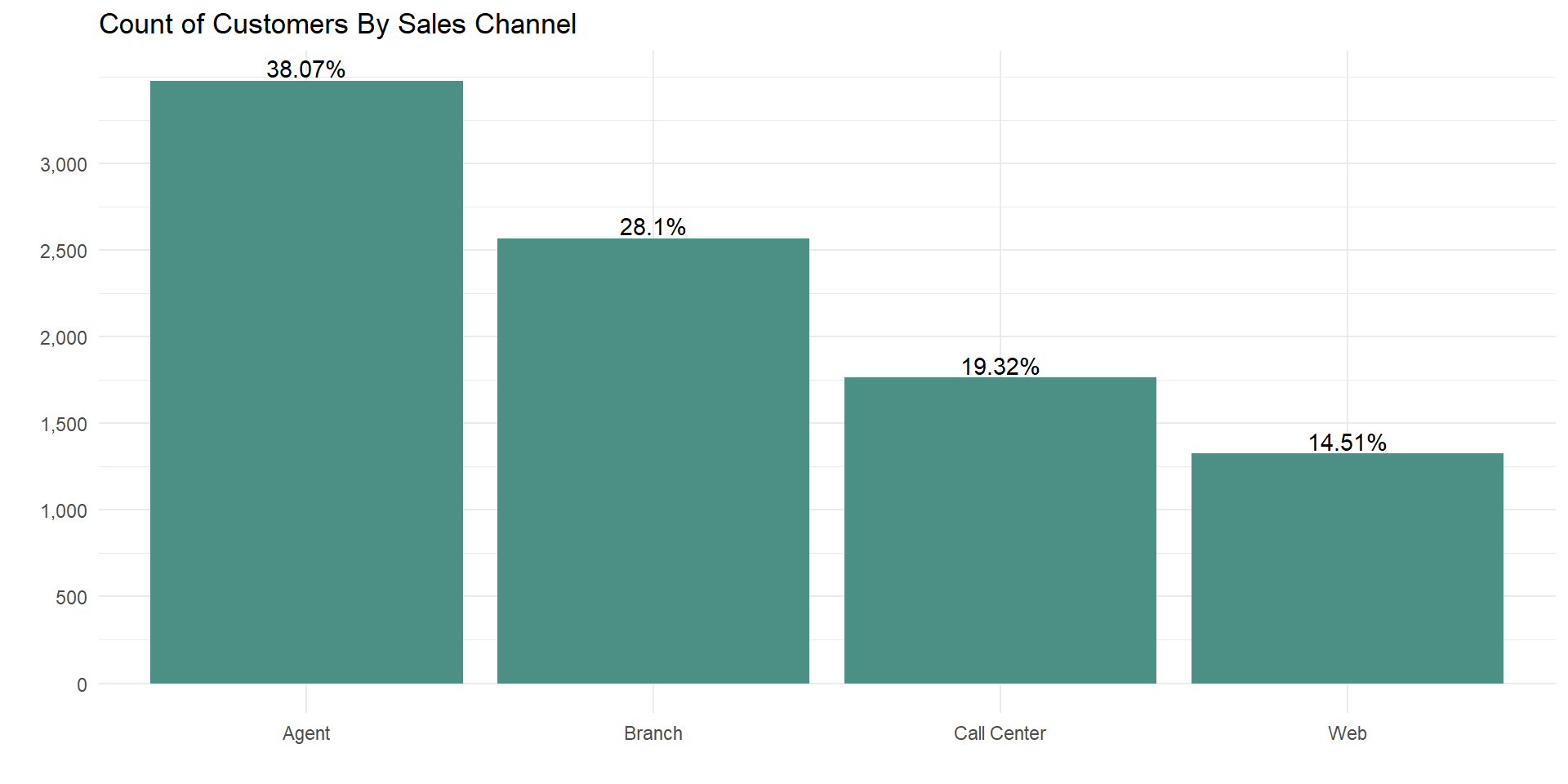 We can see that majority of the customers where acquired through auto
insurance sales agencies followed by the company’s other branches, while
less success was achieved using online platforms to acquire new
customers.
numeric_dis(data, customer_lifetime_value)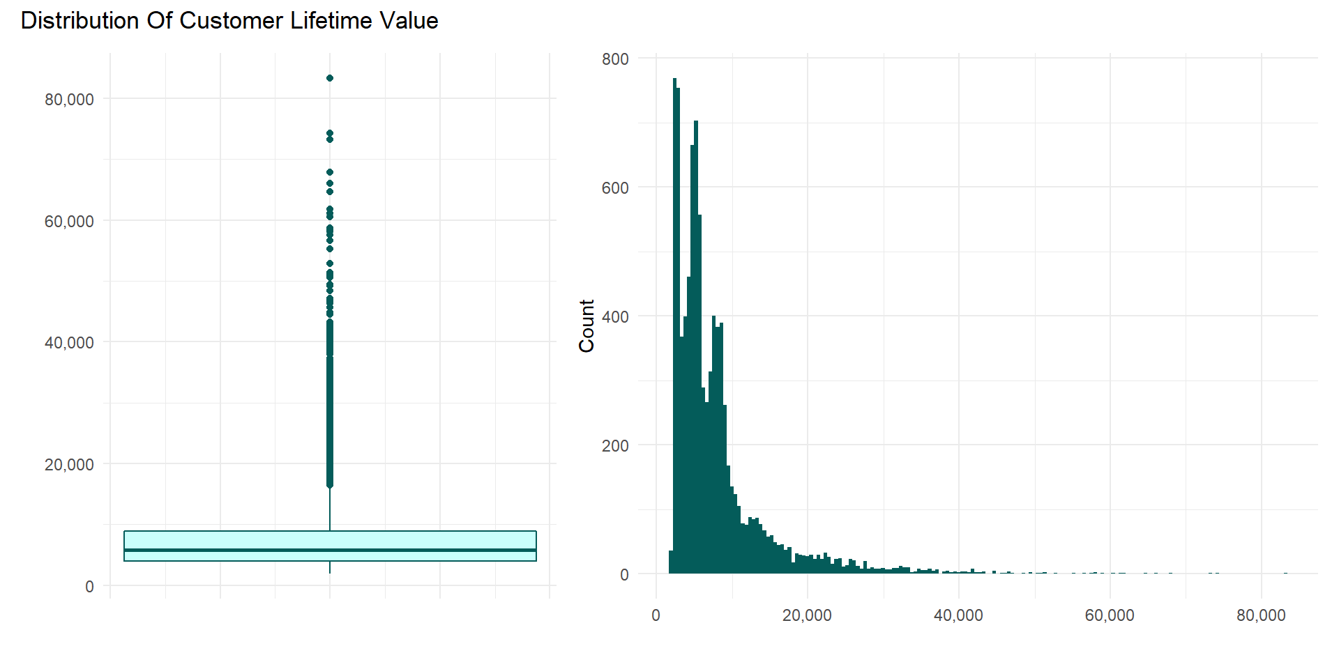
The average CLV is 5,780, Most policyholders have less than 10,000
CLV and just a few are above 40,000.
Distribution of CLV by sales channel.
num_cat_dis(data,
            customer_lifetime_value,
            sales_channel,
            outlier = "suo",
            p_typ = "box")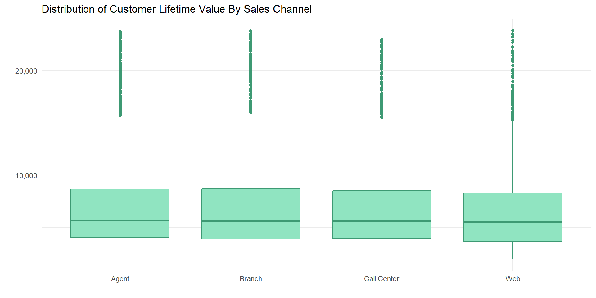
Average CLV by sales channel.
num_cat_sumy(data, customer_lifetime_value, sales_channel)
Total CLV by sales channel.
num_cat_sumy(data, customer_lifetime_value, sales_channel, sumy_fun = median)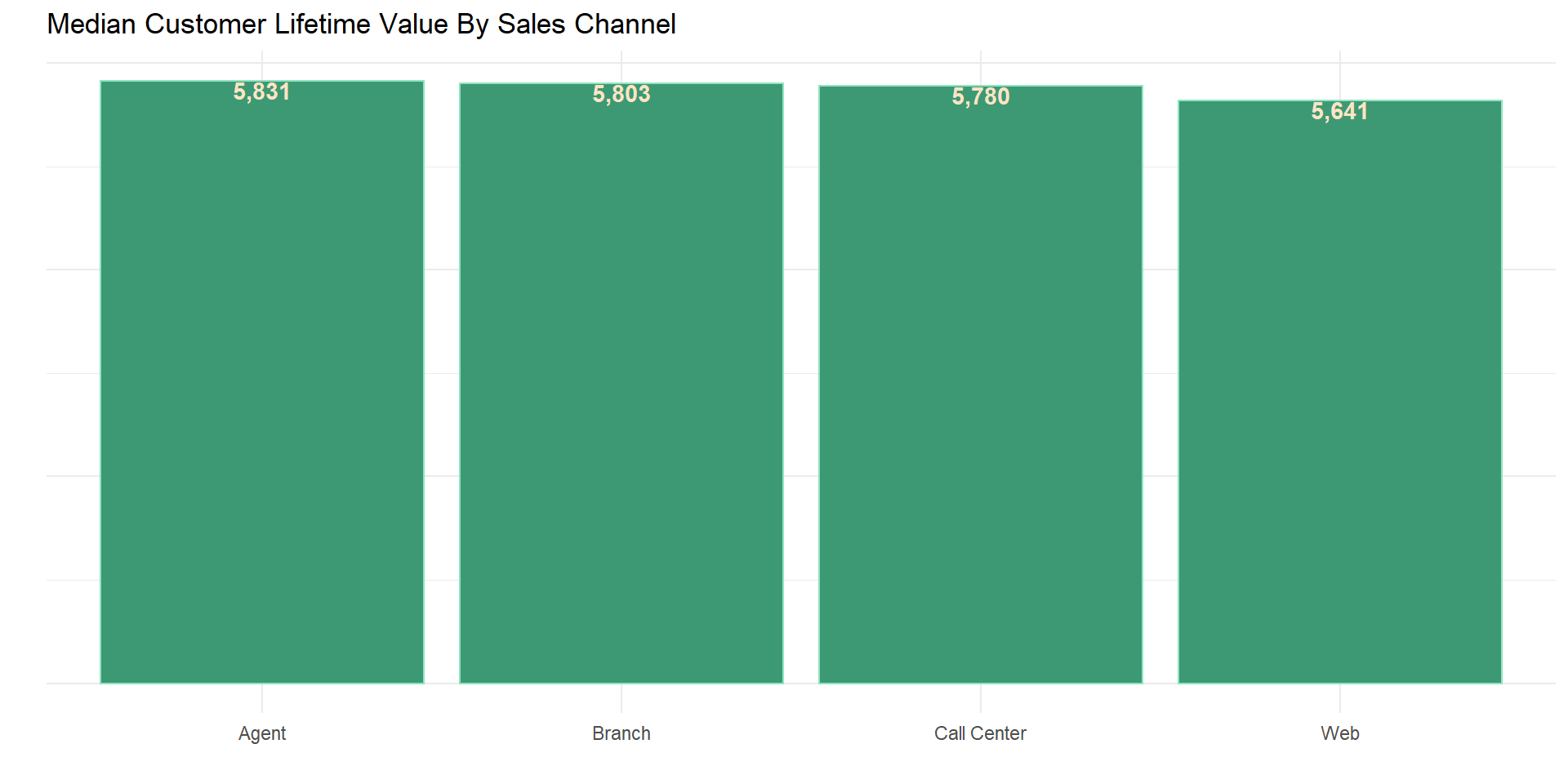
While There is a huge difference in the total CLV for all sales
channels, when we look at the median CLV there is only a slight
distinction for all channels
Customer’s income effect on CLV
numeric_dis(data, income)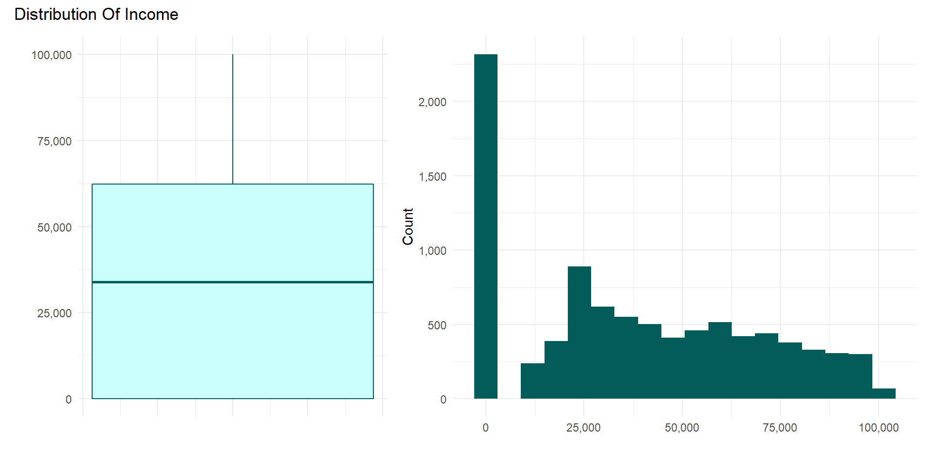
data %>%
  mutate(zero_income = if_else(income == 0, "zero income", "non-zero income")) %>%
  group_by(zero_income) %>%
  summarise(count = n(), proportion = count/nrow(data)*100)
## # A tibble: 2 × 3
## zero_income count proportion
## <chr> <int> <dbl>
## 1 non-zero income 6817 74.6
## 2 zero income 2317 25.42,317 customers which is 25.4% of the total customer have 0 income. Also fewer customers have income above 62,320.
corr_lysis(data, customer_lifetime_value, income)## # A tibble: 1 × 8
## estimate statistic p.value parameter conf.low conf.high method alter…¹
## <dbl> <dbl> <dbl> <int> <dbl> <dbl> <chr> <chr>
## 1 0.0244 2.33 0.0199 9132 0.00386 0.0449 Pearson's pro… two.si…
## # … with abbreviated variable name ¹alternativedata %>%
ggplot(aes(customer_lifetime_value, income)) +
geom_point(alpha = 0.5, color = "#65ab7c") +
scale_x_continuous(labels = scales::comma_format()) +
scale_y_continuous(labels = scales::comma_format()) +
labs(x = "Customer Lifetime Value", y = "Income") +
ggtitle("Relationship Between Customer Income & CLV") +
theme_minimal()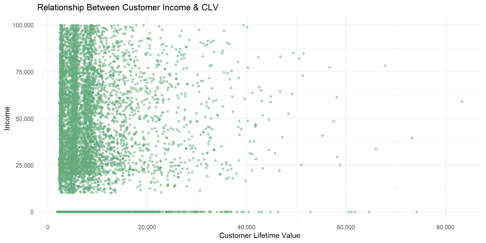
There is a weak positive correlation between customer income and CLV,
we can’t be certain that customers with high income are not majorly
buying more auto policy than customers with low income as there are
other major factors influencing this relationship.
The relationship between CLV and number of policy owned.
data_np <- data %>%
  select(number_of_policies, customer_lifetime_value) %>%
  mutate(number_of_policies = as.character(number_of_policies))

count_obs(data_np, number_of_policies)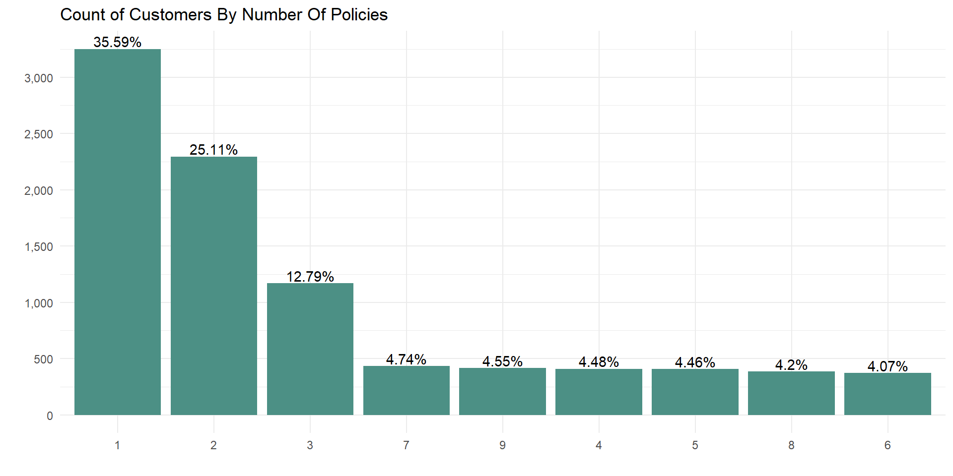
The above plot shows that there are more customers with 7 and 9 number policies than customers with 4 and 5, the top three number of policy owned by customers are 1, 2 and 3 which is not surprising.
num_cat_sumy(data_np, customer_lifetime_value, number_of_policies)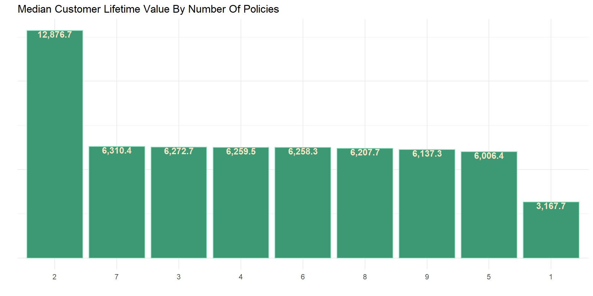
More customers with a high (above 20,000) CLV have 2 types of policy. Customers with just 1 policy have the lowest median CLV while customers with 7 policies have the second highest CLV.
Locations of the company most valuable customers.
State analysis
count_obs(data, state)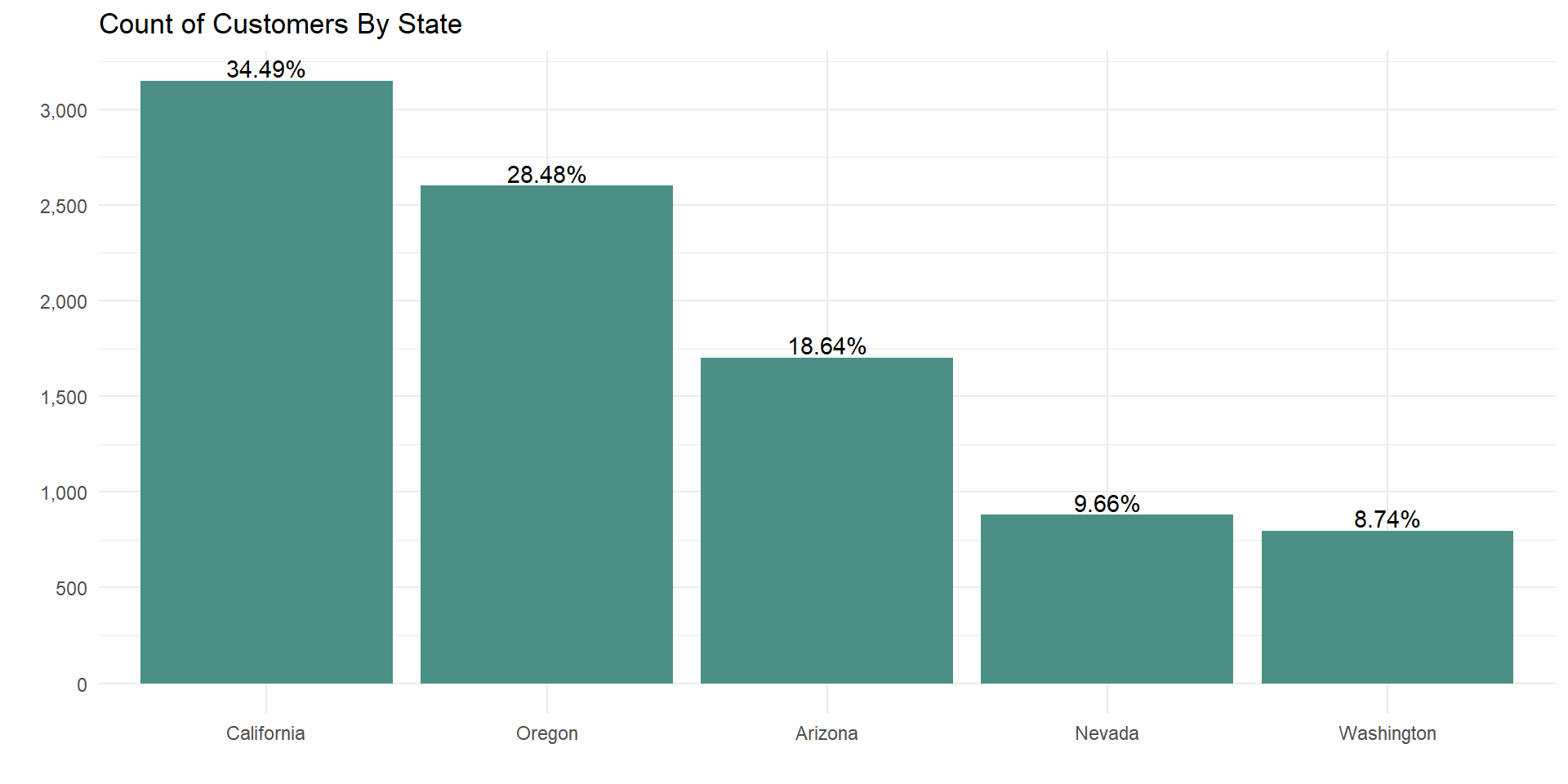
num_cat_sumy(data, customer_lifetime_value, state)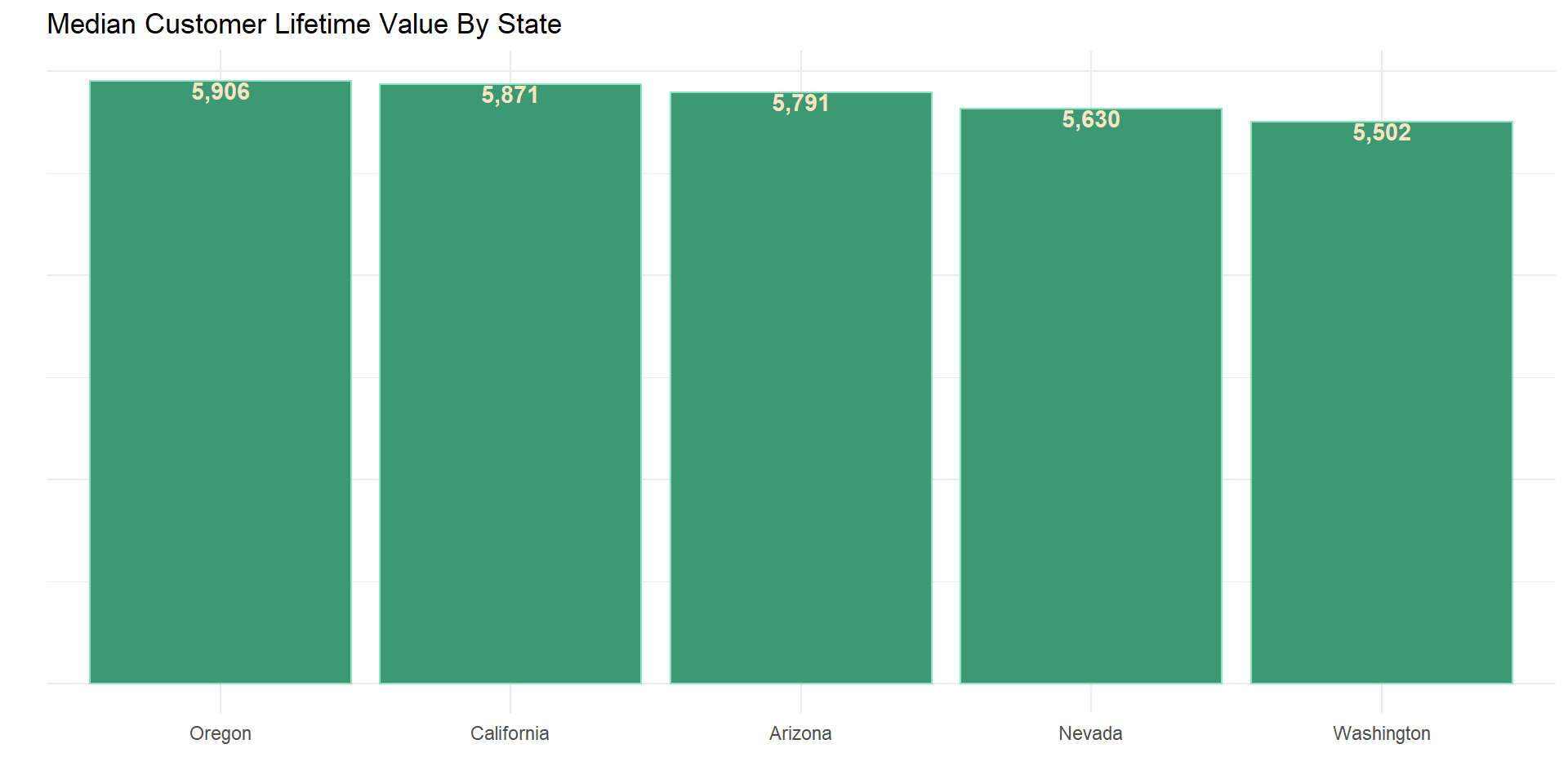
num_cat_sumy(data, customer_lifetime_value, state, p_typ = "min_max")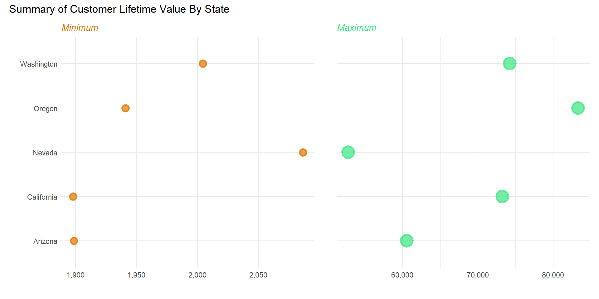
The count shows the top three state with the most market share are California, Oregon, and Arizona.
Location code analysis.
count_obs(data, location_code)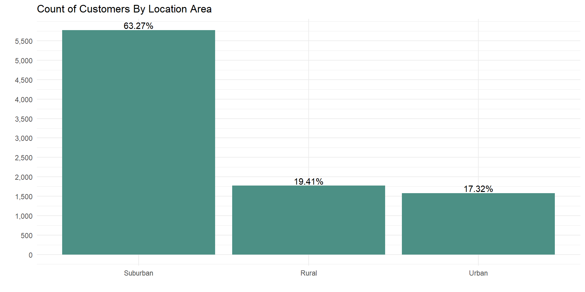
num_cat_dis(data, customer_lifetime_value, location_code, p_typ = "fqp")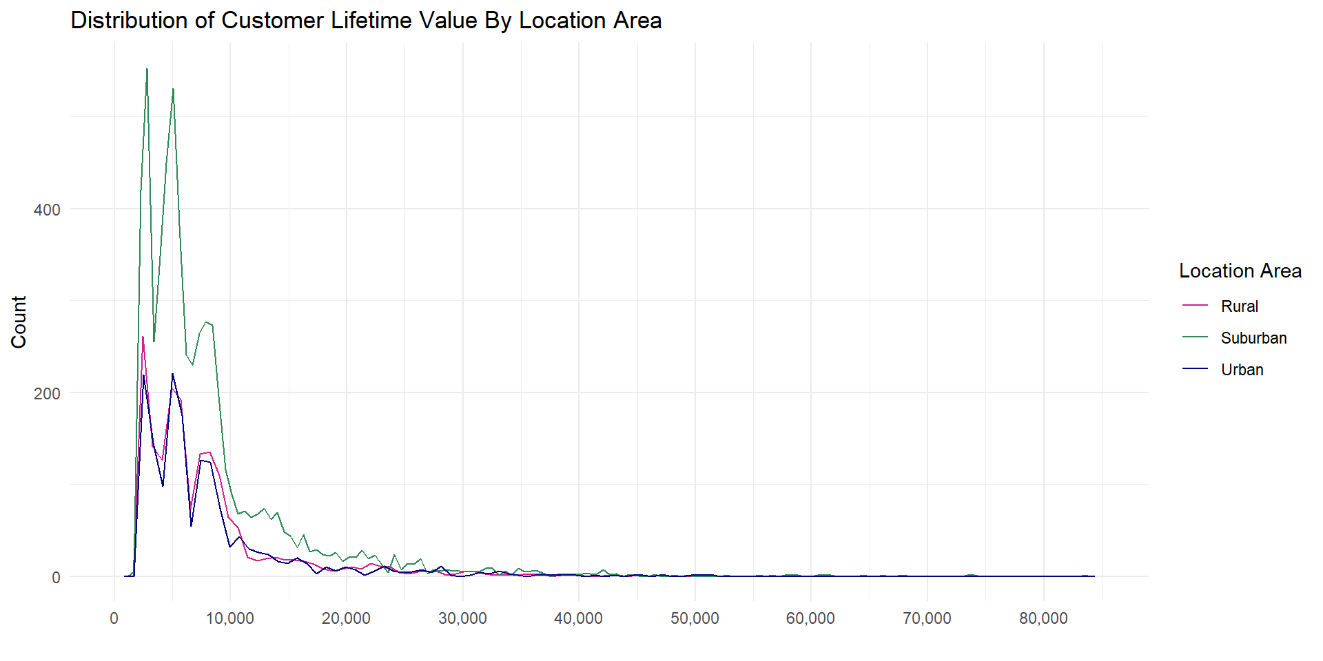
num_cat_sumy(data, customer_lifetime_value, location_code)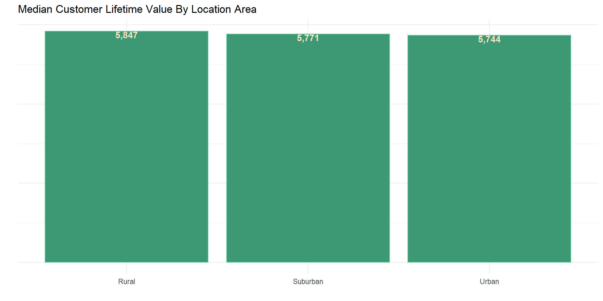
Removing outliers.
num_cat_sumy(data, customer_lifetime_value, location_code, outlier = "uo")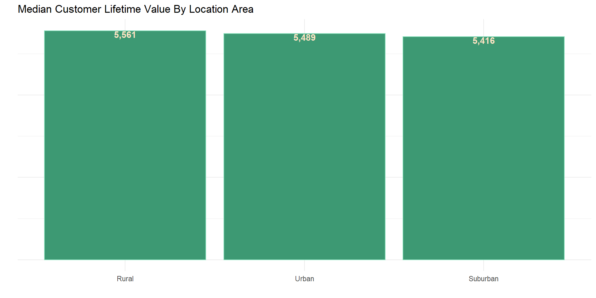
num_cat_sumy(data, customer_lifetime_value, location_code, p_typ = "min_max")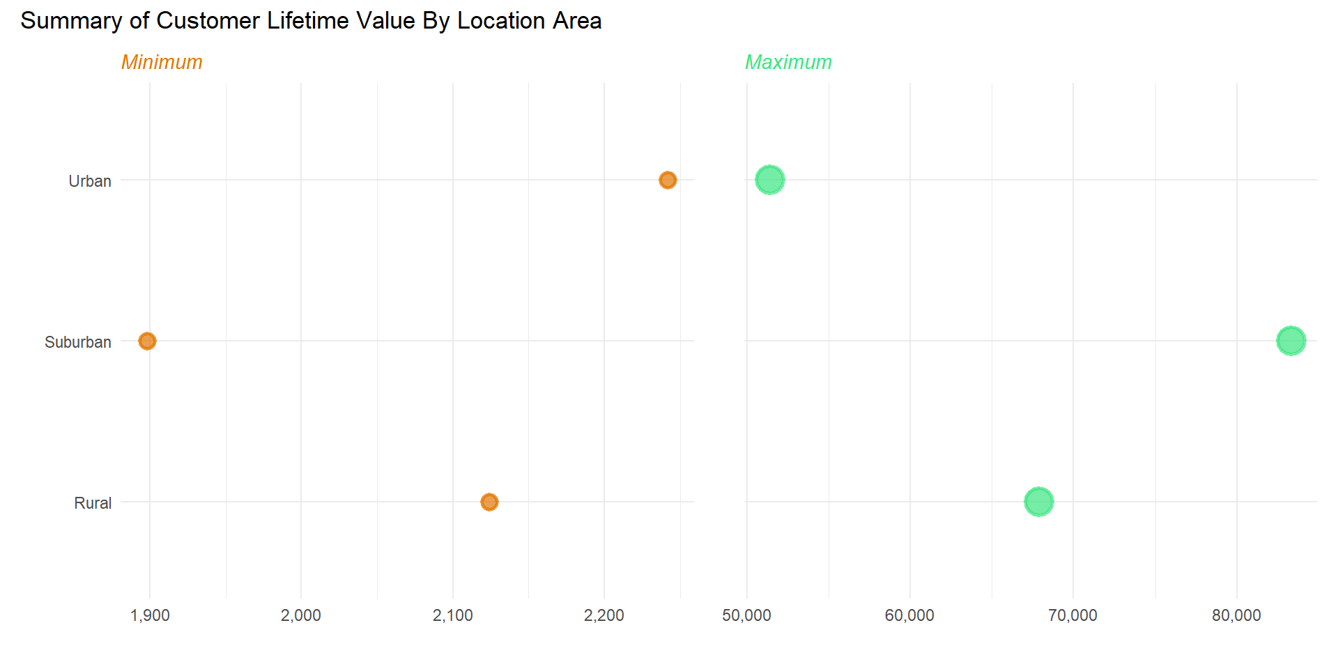
More customers leave in suburban than rural and urban areas, while
urban dwellers are the least majority group.
For all the three location area most customers have low CLV than high
CLV but rural dwellers have the highest median CLV.
Joint analysis
count_obs2(data, state, location_code)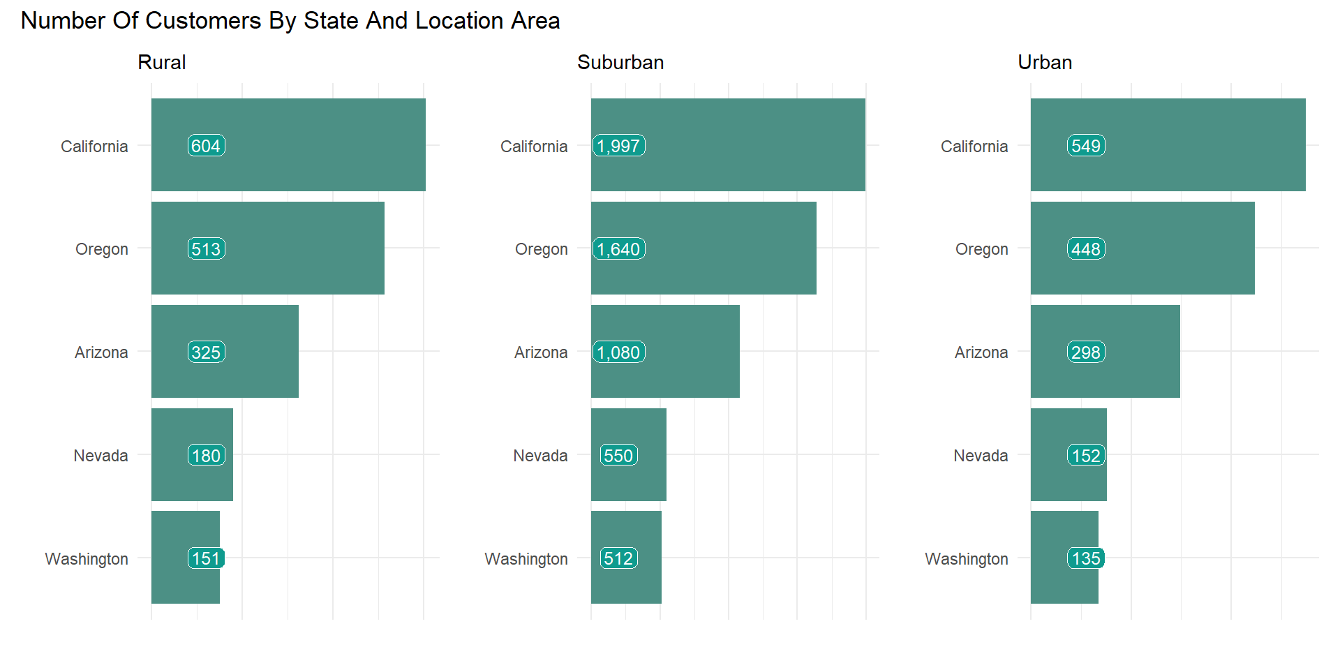
num_cat_sumy2(data,
              customer_lifetime_value,
              state,
              location_code,
              txt_pos = 1500)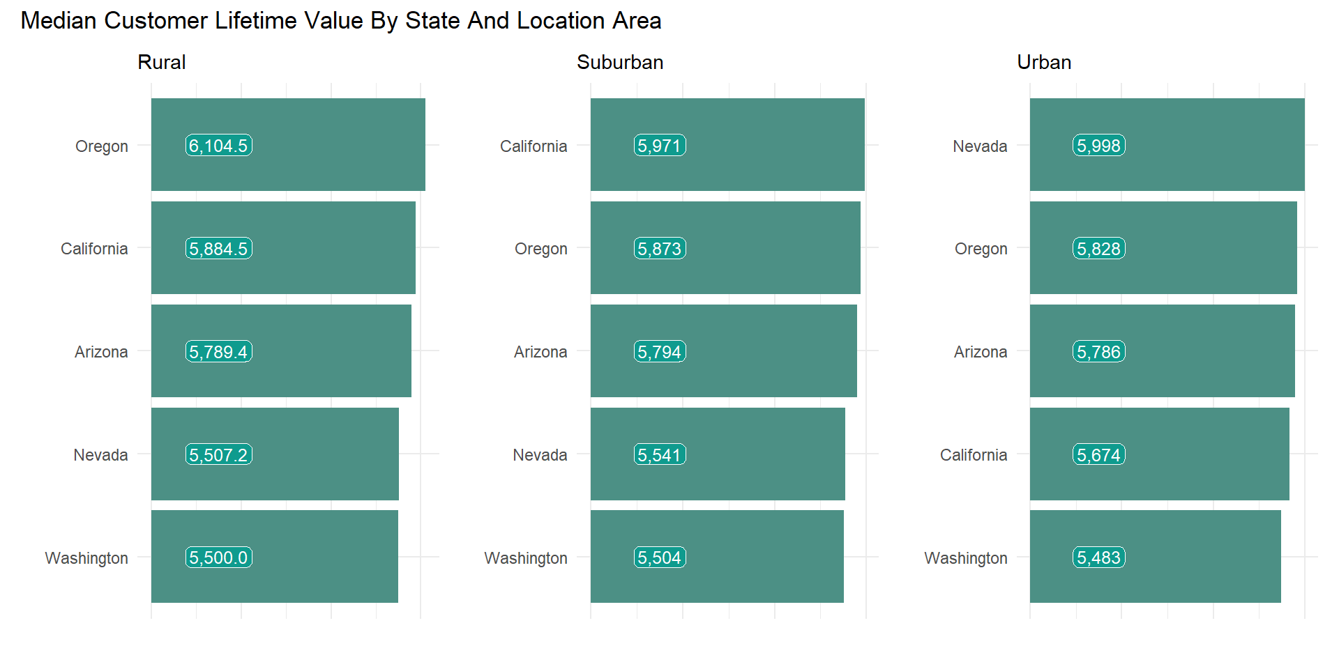
The most valuable customers leaving in Rural area can be found in Oregon. In Suburban area California has the highest average CLV. While in Urban area most valuable customers leave in Nevada.
Previous Set Up
Next Various Features Used In Determining Auto
Premium