Various Features Used In Determining Auto Premium
Relationship between total claim amount and Premium
Correlation
corr_lysis(data, monthly_premium_auto, total_claim_amount)## # A tibble: 1 × 8
## estimate statistic p.value parameter conf.low conf.high method alter…¹
## <dbl> <dbl> <dbl> <int> <dbl> <dbl> <chr> <chr>
## 1 0.632 77.9 0 9132 0.620 0.644 Pearson's pro… two.si…
## # … with abbreviated variable name ¹alternativenumerical_rel(data,
monthly_premium_auto,
total_claim_amount, p_typ = "bin2d")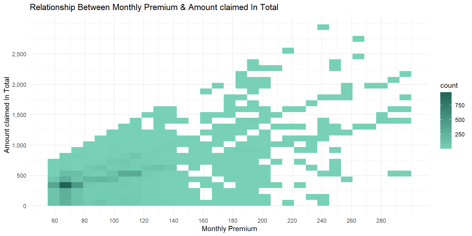
There is a moderate positive correlation (0.632) between the total amount claimed by customers and the amount of premium paid on a monthly basis. There is a large number of customers that have less than 500 claim amount pays less than 80 premium monthly.
Relationship between coverage and Premium
num_cat_dis(data, monthly_premium_auto, coverage)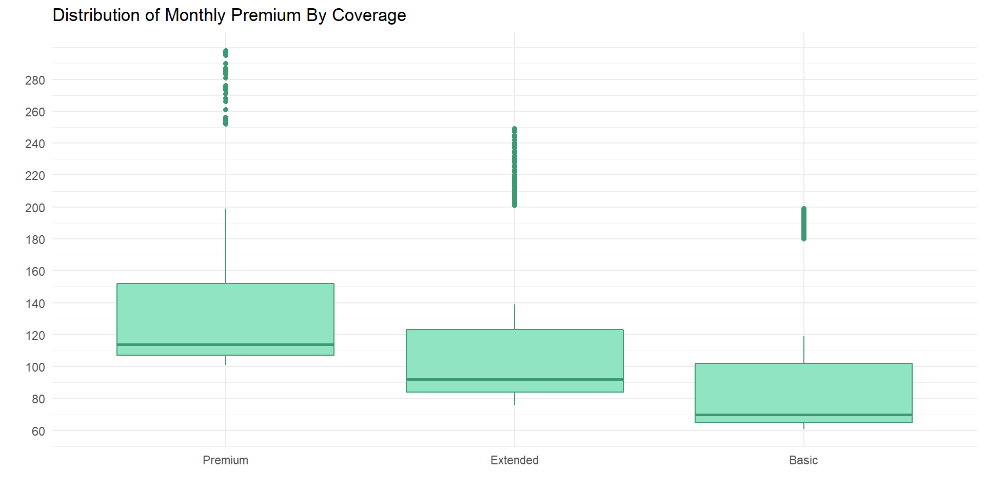
num_cat_sumy(data, monthly_premium_auto, coverage)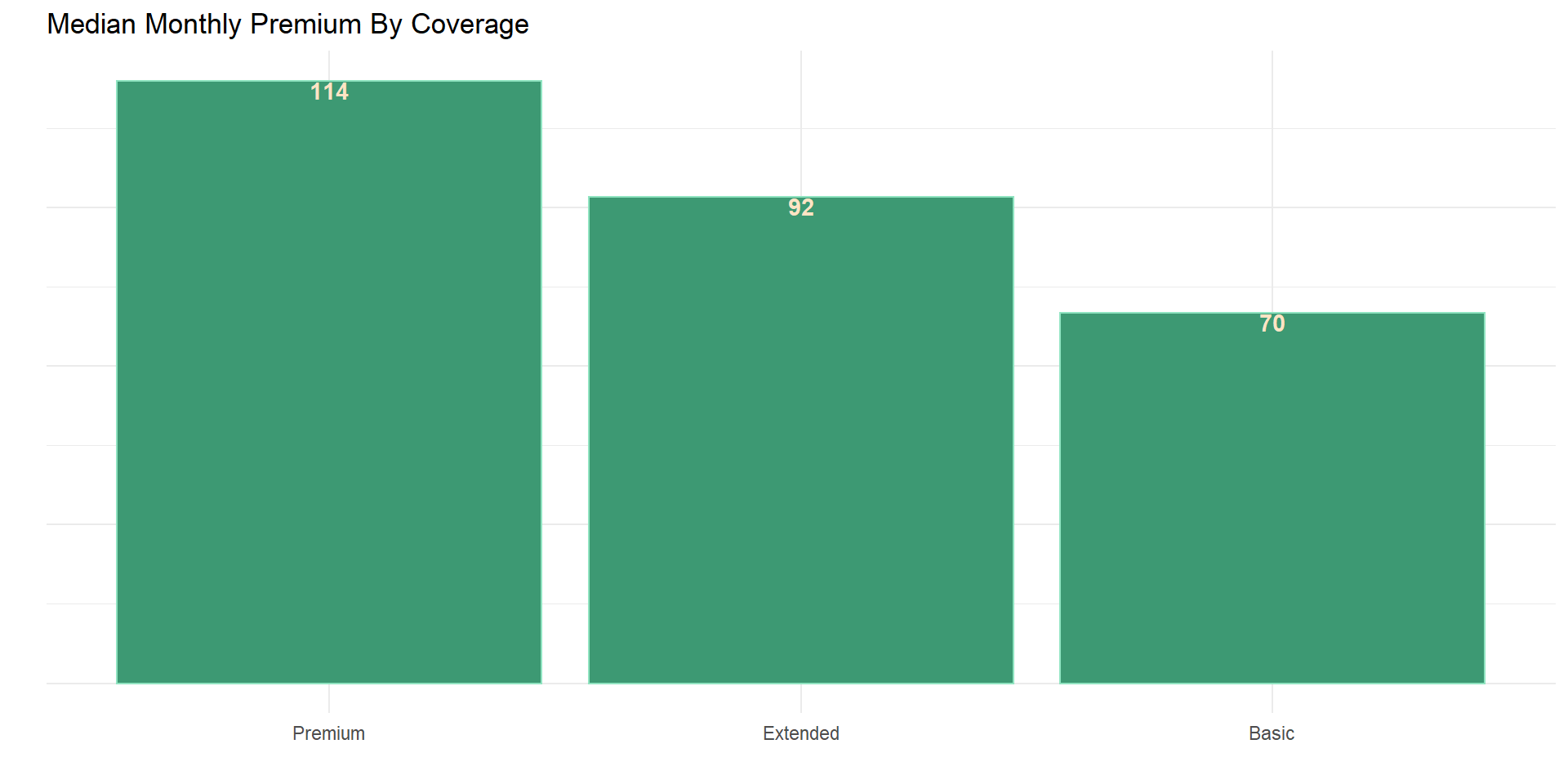
num_cat_sumy(data, monthly_premium_auto, coverage, sumy_fun = sum)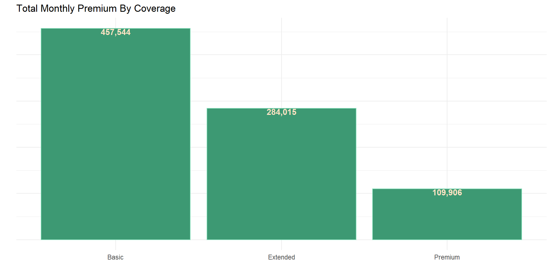
The higher the level of coverage the more the average monthly premium that was paid.
Relationship between driver profile and Premium
Marital status
num_cat_sumy(data, monthly_premium_auto, marital_status)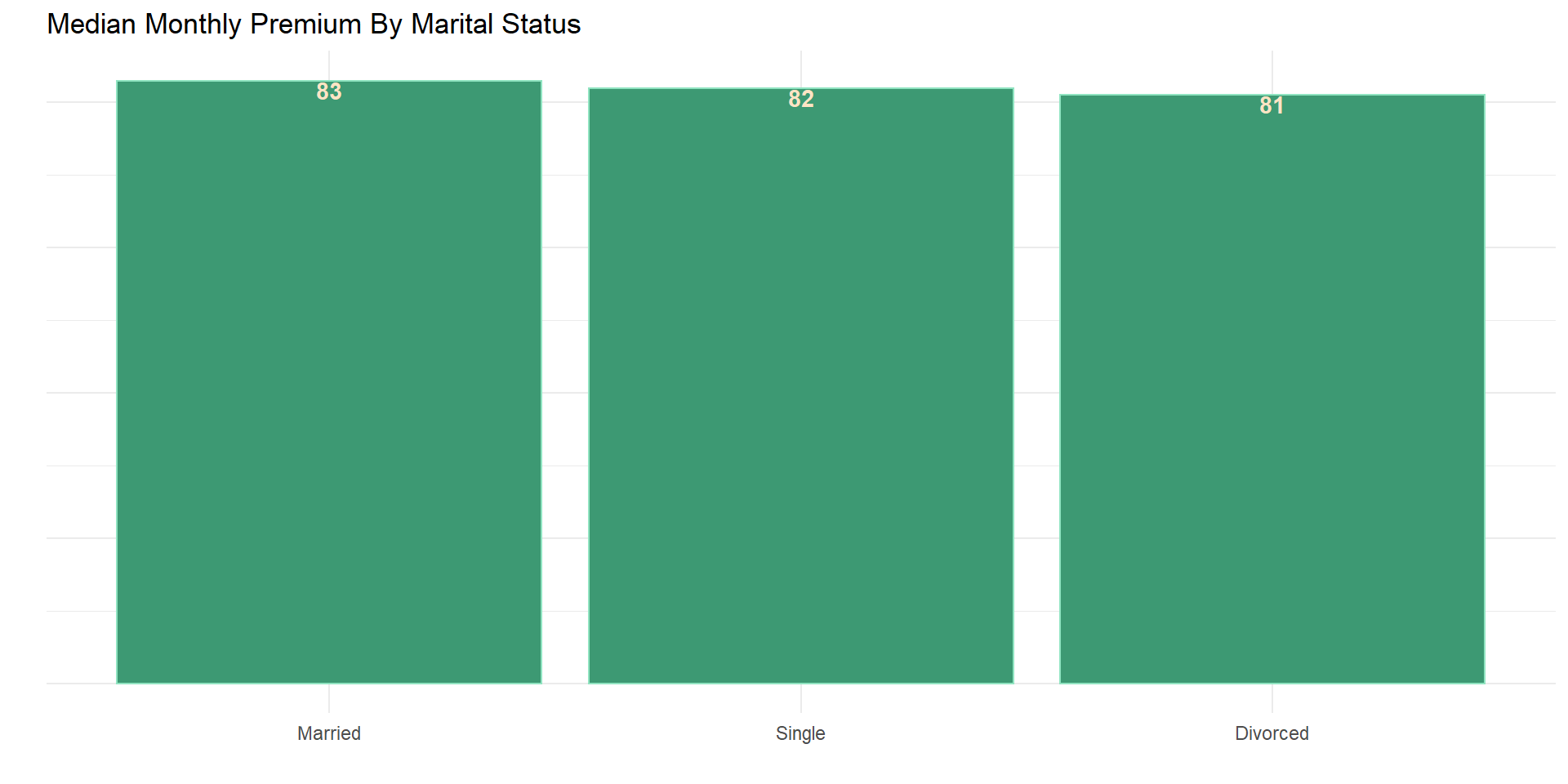
There is a slight distinction in the median premium paid monthly between married (83.0), Single (82.0) and Divorced (81.0) customers.
Gender
num_cat_dis(data, monthly_premium_auto, gender, p_typ = "fqp")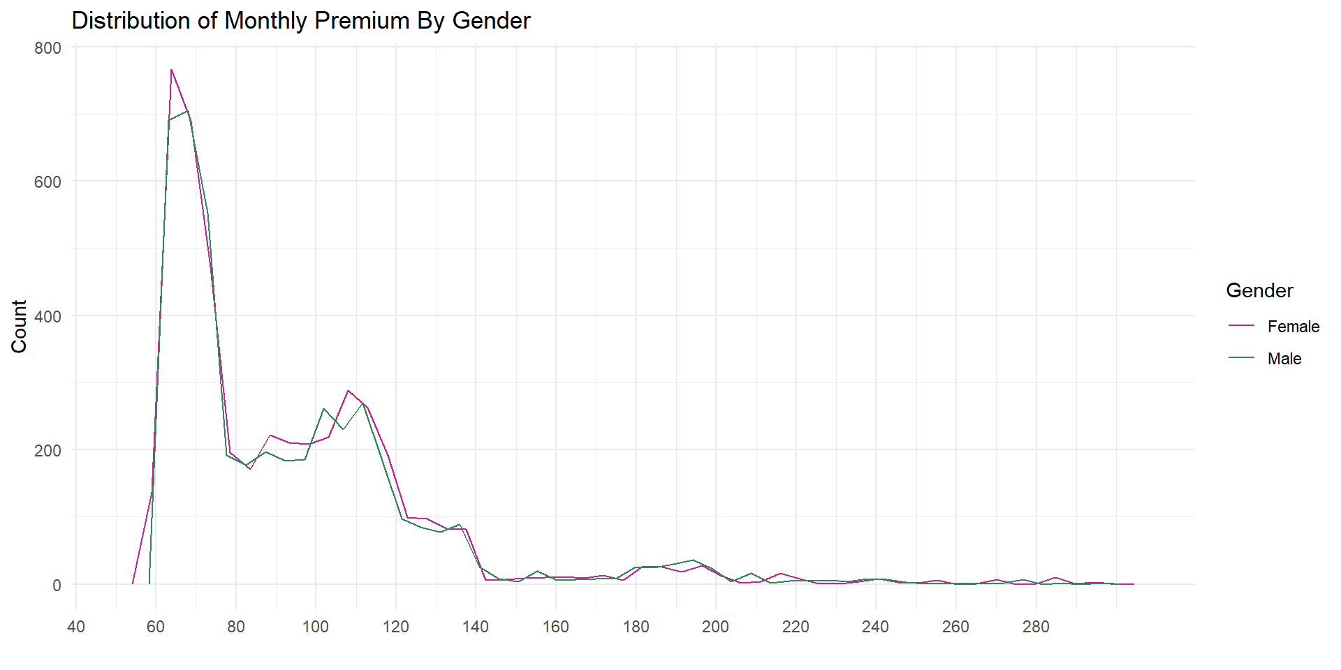
num_cat_sumy(data, monthly_premium_auto, gender, sumy_fun = sum)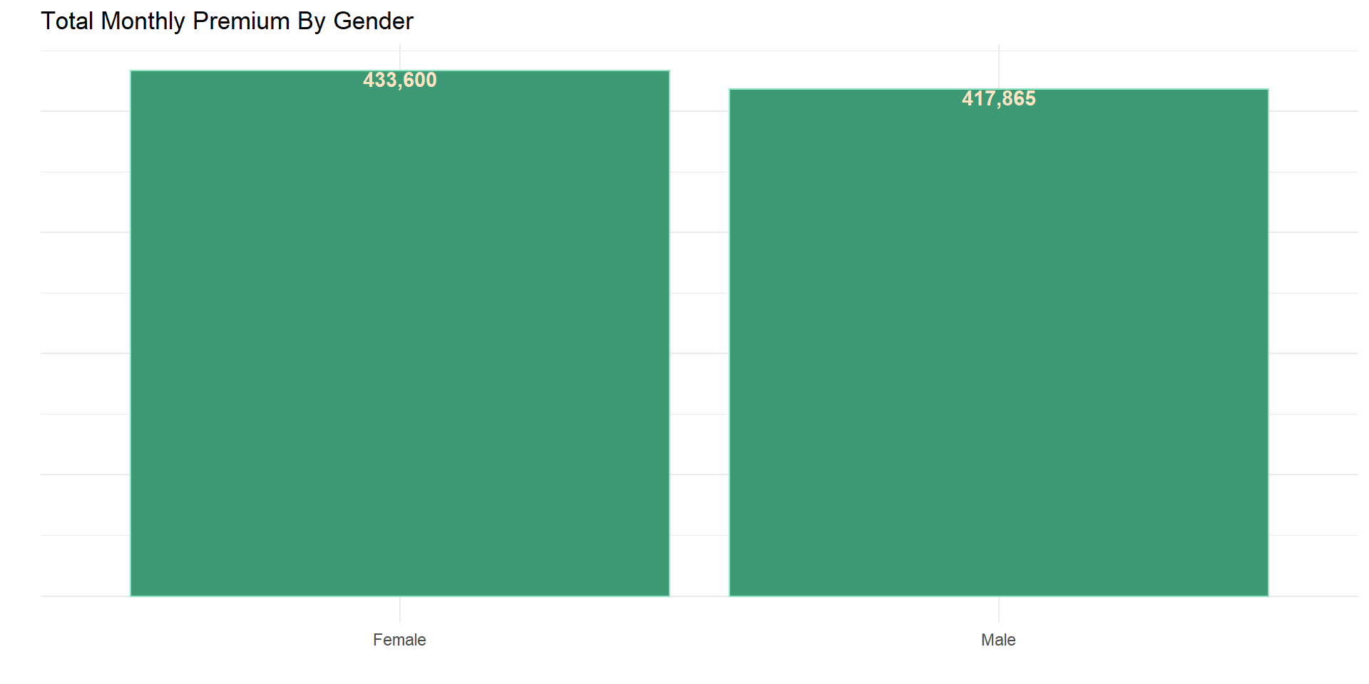
Female customers paid more premium (433,600) than male customers (417,865) but on an average there is a little difference in the amount of premium paid.
num_cat_sumy2(data, monthly_premium_auto, marital_status, gender)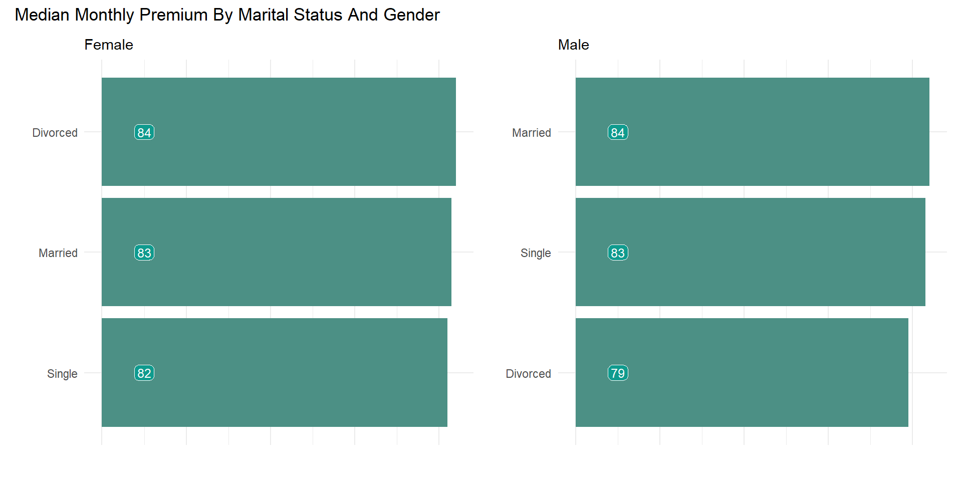
g_ms <- data %>%
  group_by(marital_status, gender) %>%
  numeric_summary(monthly_premium_auto)

g_ms_f <- filter(g_ms, gender == "Female")
g_ms_m <- filter(g_ms, gender == "Male")

ggplot(g_ms, aes(y = marital_status, fill = gender)) +
  geom_col(data = g_ms_f, aes(x = sum), color = "white") +
  geom_col(data = g_ms_m, aes(x = -1*sum), color = "white") +
  geom_text(data= g_ms_f, aes(label=scales::comma(sum), x=sum), hjust= 1.3) +
  geom_text(data= g_ms_m, aes(label=scales::comma(sum), x=-1*sum), hjust= -0.5) +
  theme(axis.text.x = element_blank()) +
  scale_fill_manual(values = c("#0bf9ea", "#029386")) +
  theme_minimal() +
  labs(x = "", y = "", fill = "Gender",
       title = "Total Monthly Premium by Marital Status & Gender")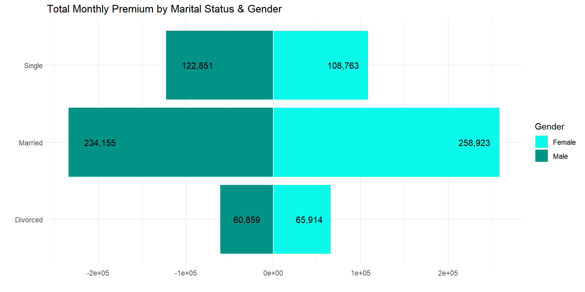
In total, married customers paid the largest chunk of premium for both male and female followed by Single customers than divorced customers.Whereas on an average divorced female customers paid more premium than married and single female customers while married male customers paid more premium than both single and divorced customers.
Relationship between customer’s residence and Premium
State
num_cat_sumy(data, monthly_premium_auto, state)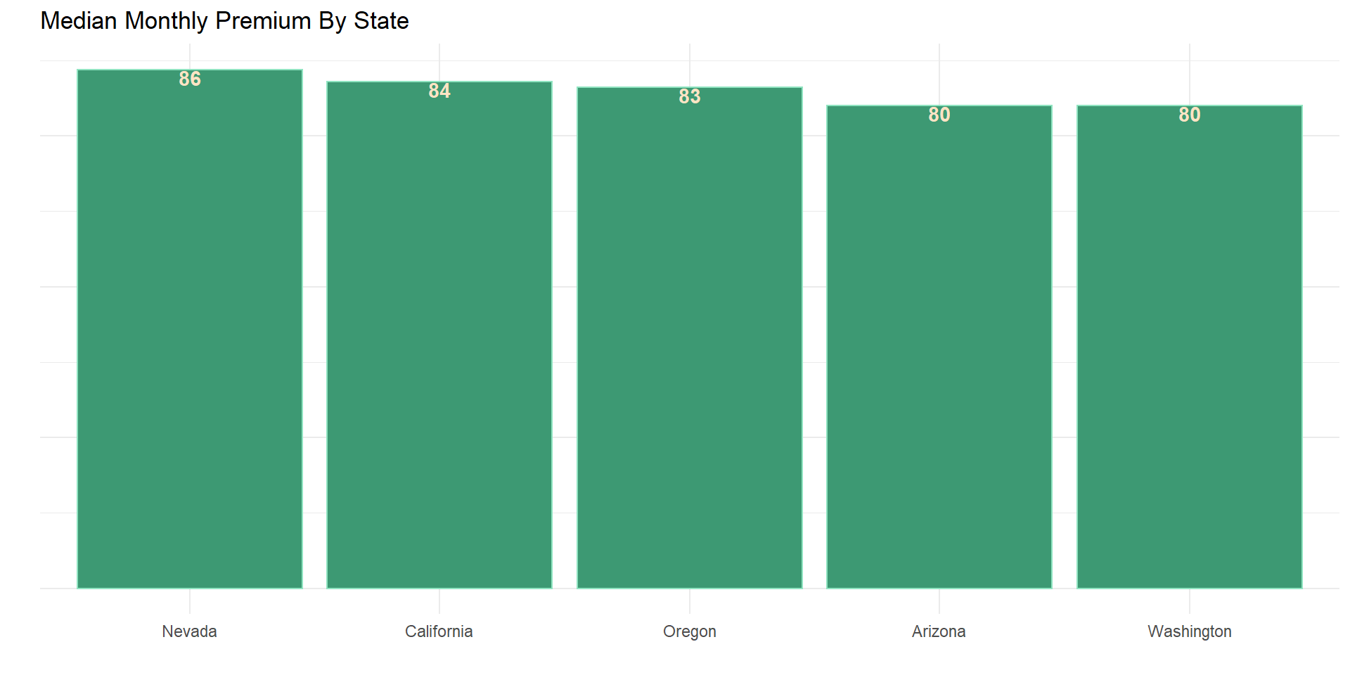
num_cat_sumy(data, monthly_premium_auto, state, sumy_fun = sum)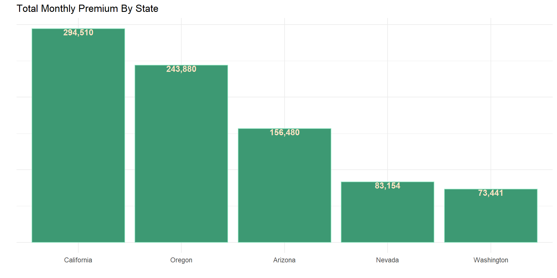
Total Monthly premium paid is the highest in California followed by Oregon and Arizona this is boosted by the market share of customers in those state. While based of the median monthly premium, customers in Nevada paid more premium monthly, which is directly followed by California and Oregon.
Location Code
num_cat_sumy(data, monthly_premium_auto, location_code)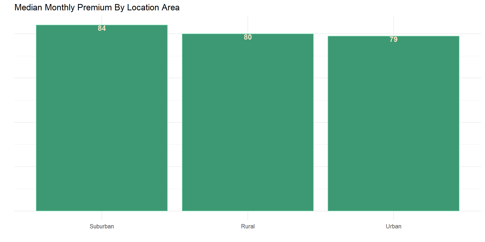
num_cat_sumy(data, monthly_premium_auto, location_code, sumy_fun = sum)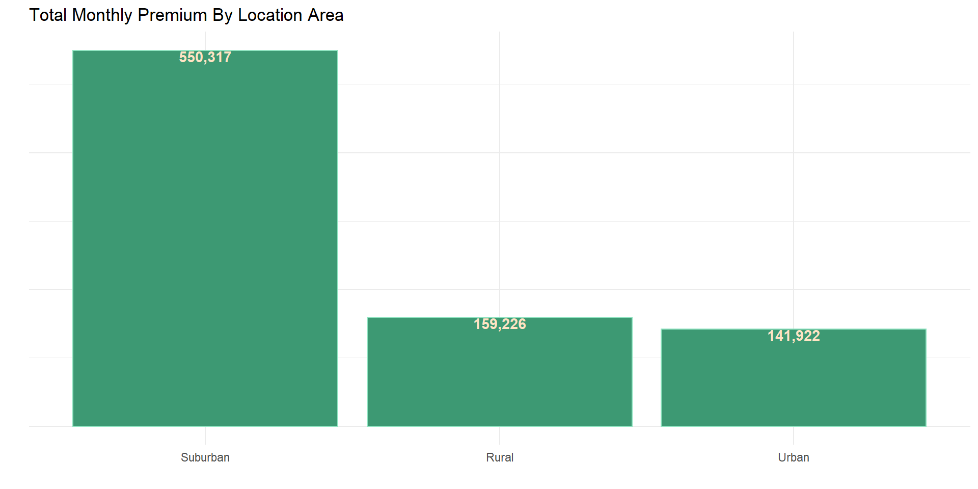
Given that safe areas pays less premium than area that are known to be unsafe, the analysis shows that Urban customers pays less premium when looking at the median monthly premium than rural and suburban customers. In essence there is a possibility that the company perceived that Suburban areas are less safe for vehicle than rural and urban areas.
num_cat_sumy2(data, monthly_premium_auto, state, location_code)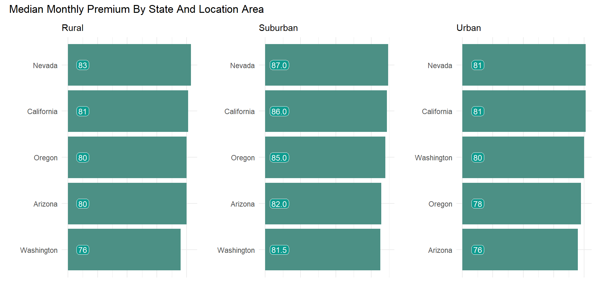
Given the relationship between premium and customer’s state above, urban areas pay less premium than rural and suburban with the exception of Washington where customers paid a higher premium in urban areas than rural areas.
Relationship between vehicle classification and Premium
Vehicle class
num_cat_dis(data, monthly_premium_auto, vehicle_class, p_typ = "vio")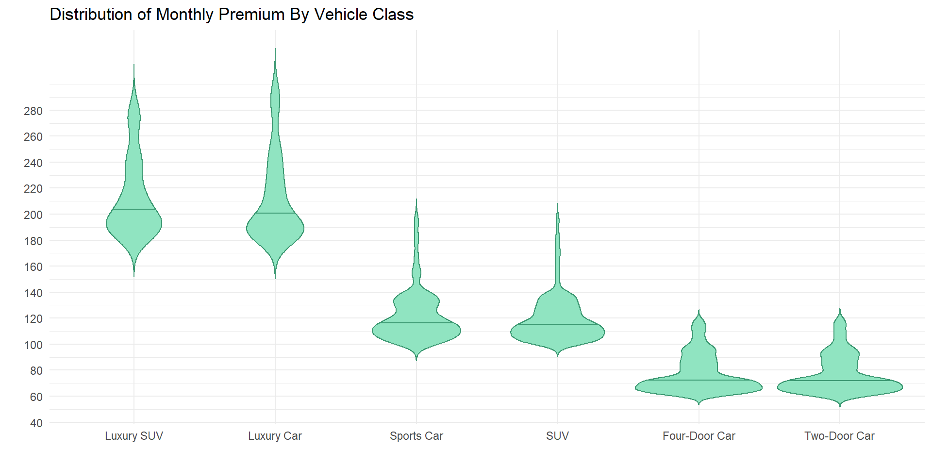
num_cat_sumy(data, monthly_premium_auto, vehicle_class)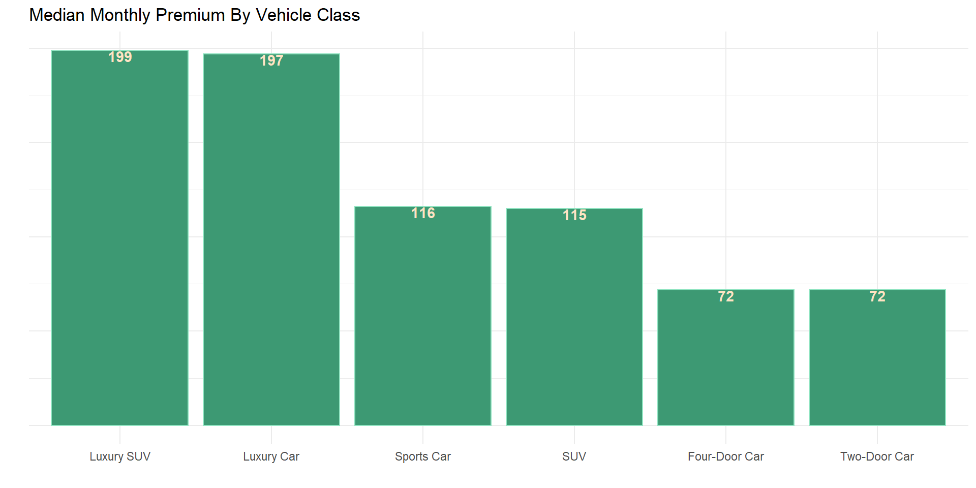
vehicle known for their higher quality and class cost more premium than other classes of vehicles, from the analysis it shows that owners of luxury SUV, luxury cars and sport cars paid more premium on an average than other vehicle class.
Vehicle size
num_cat_dis(data, monthly_premium_auto, vehicle_size, p_typ = "vio")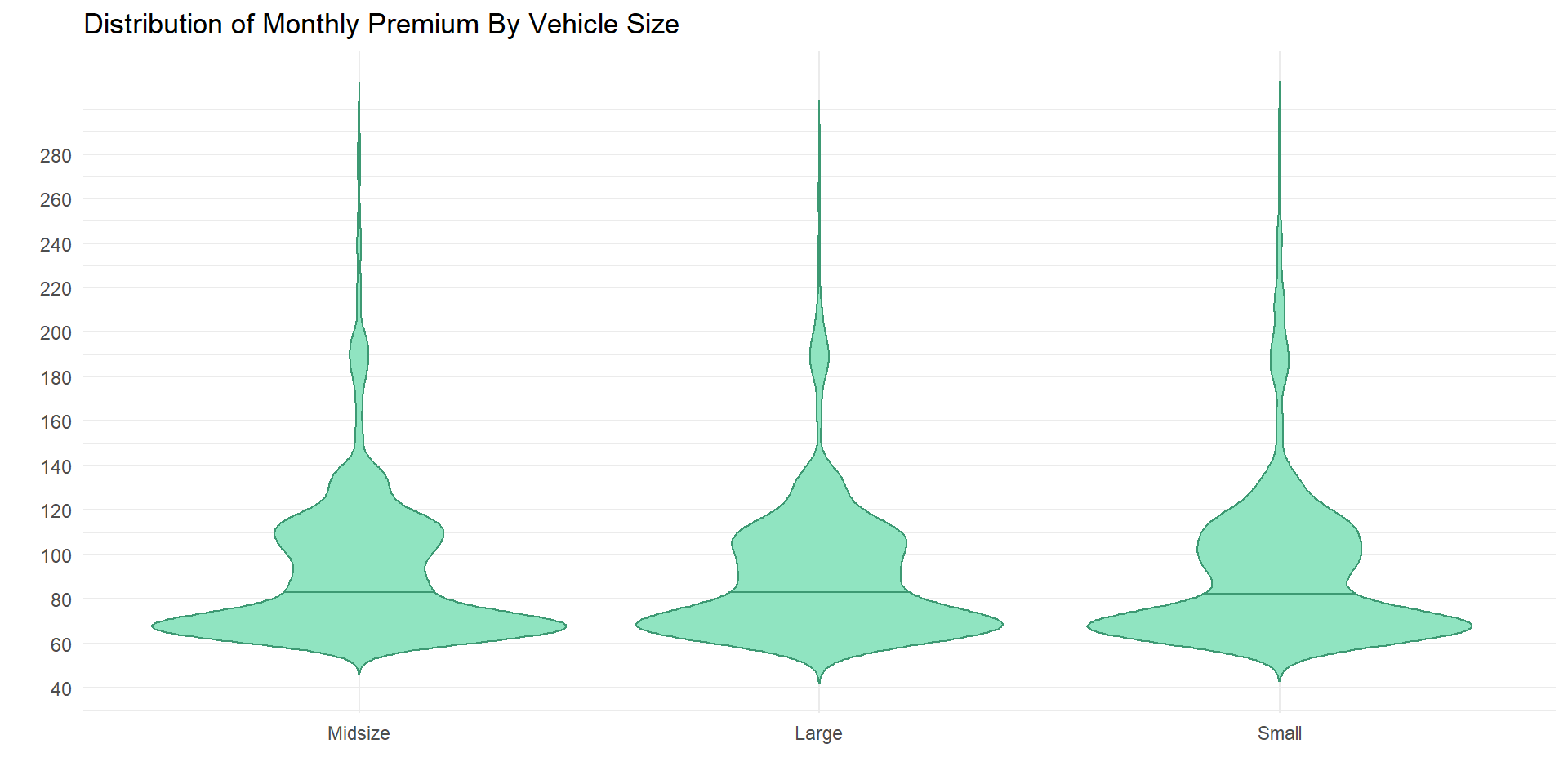
num_cat_sumy(data, monthly_premium_auto, vehicle_size)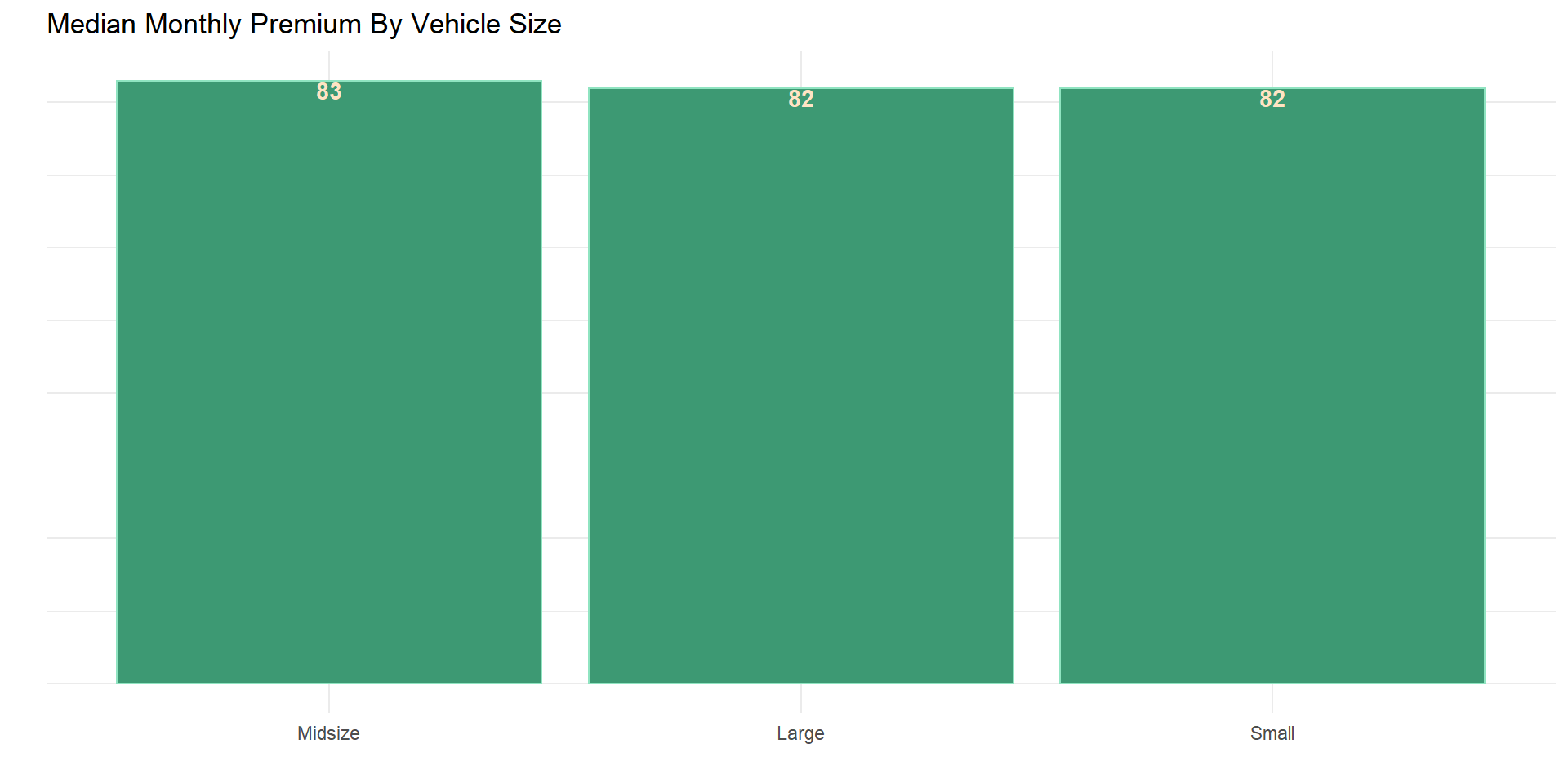
Customers with midsize vehicles paid more premium on an average than customer with large vehicles and small vehicles (there is a large segment or customers with midsize vehicles).
num_cat_sumy2(data, monthly_premium_auto, vehicle_size, vehicle_class)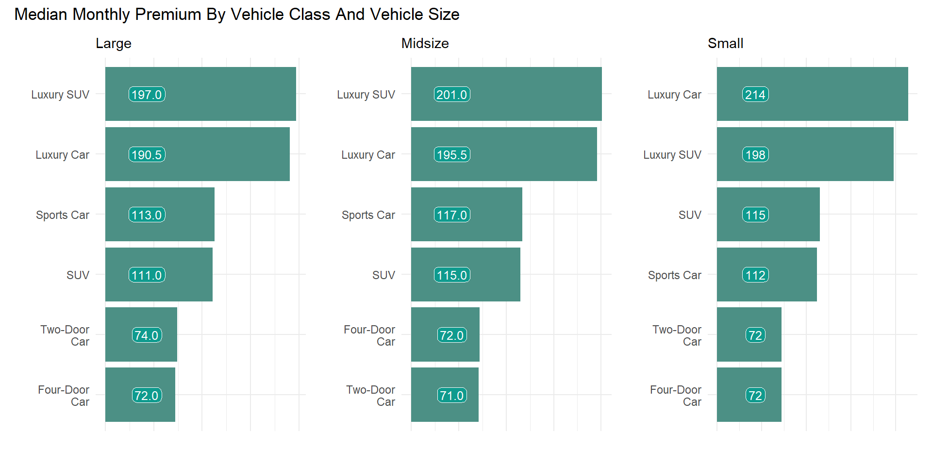
Given the above analysis on both vehicle class and size, higher quality cars pays more for all vehicle size with the exception of small size Sport Car which paid less premium than small size SUV.
Previous Analysis on Customer Lifetime
Values
Next Analysis On Number Of Policies Owned By
policyholders